Tutorial

Overview

Welcome to MPicker! To install the software, refer to the Installation and Download pages. For detailed information about the GUI, consult the Manual page. Explore the Advanced Tutorial for tasks such as flattening complex surfaces in mesh, automatic particle picking, and Class2D. Before exploring other tutorial sections, make sure to finish the basic usage part.

Basic usage

This tutorial guides through the process of flattening membranes in the cyanobacterium Anabaena. Download the tutorial file MPicker_tutorial_v1.0.0.tar.bz2 to a directory of choice and extract it:

tar -jxvf MPicker_tutorial_v1.0.0.tar.bz2
cd tutorial

The tutorial includes three files:

• emd13771_isonet.mrc: CryoET data from EMD-13771, processed by isonet and cropped to a small size.
• seg_post_id0_thres_0.60_gauss_0.50_voxel_150.mrc: Membrane segmentation of emd13771_isonet.mrc. This can also be generated using MPicker.
• manual_surf.txt: Manually picked points used to label a membrane, demonstrating how to flatten a membrane without segmentation.

Load the data

Activate the conda environment and ensure that mpicker/mpicker_gui is in the $PATH. Open MPicker:

Mpicker_gui.py &

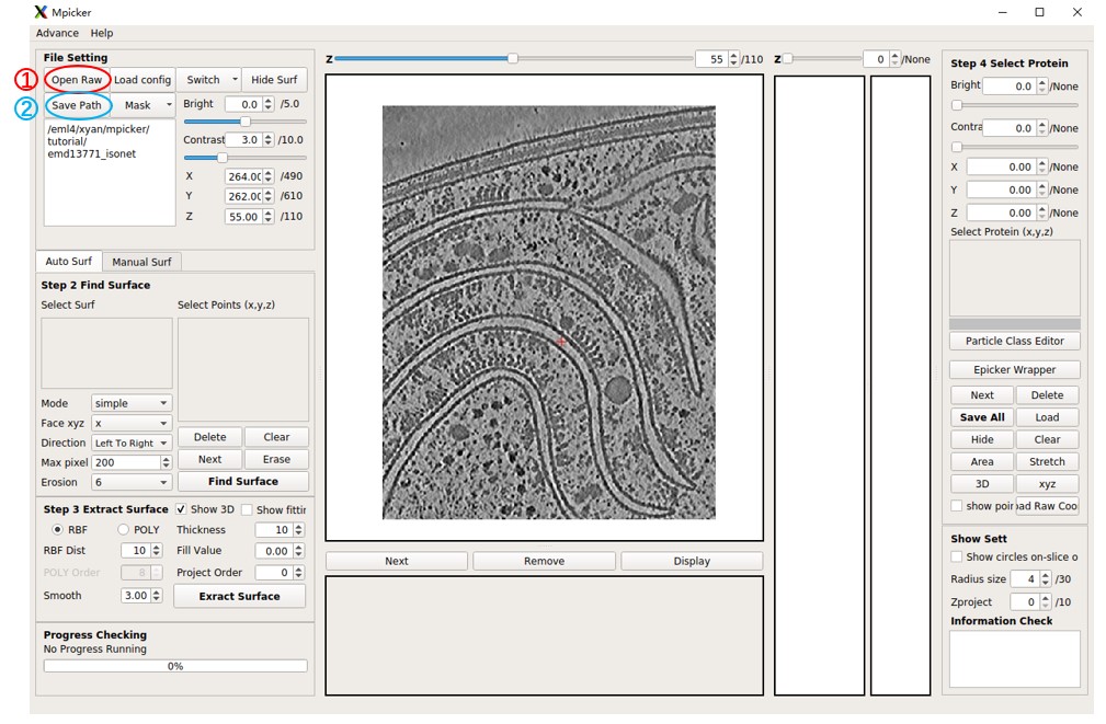
Press Open Raw and select emd13771_isonet.mrc to load it. Use mouse actions to navigate (drag to move, mouse wheel to zoom), and adjust image contrast via the spinbox of Bright and Contrast. Display xy slices at different z positions by scrolling the mouse wheel over the spinbox of z or dragging the bar.

Press Save Path and choose a folder to save the result (e.g., the current path xxx/tutorial). MPicker will create a folder xxx/tutorial/emd13771_isonet to save the result for this tomogram, and a file xxx/tutorial/emd13771_isonet.config for reloading the project later.

Load membrane segmentation

While a segmentation is provided, it can also be generated in MPicker. Refer to the Generate membrane segmentation section for details.

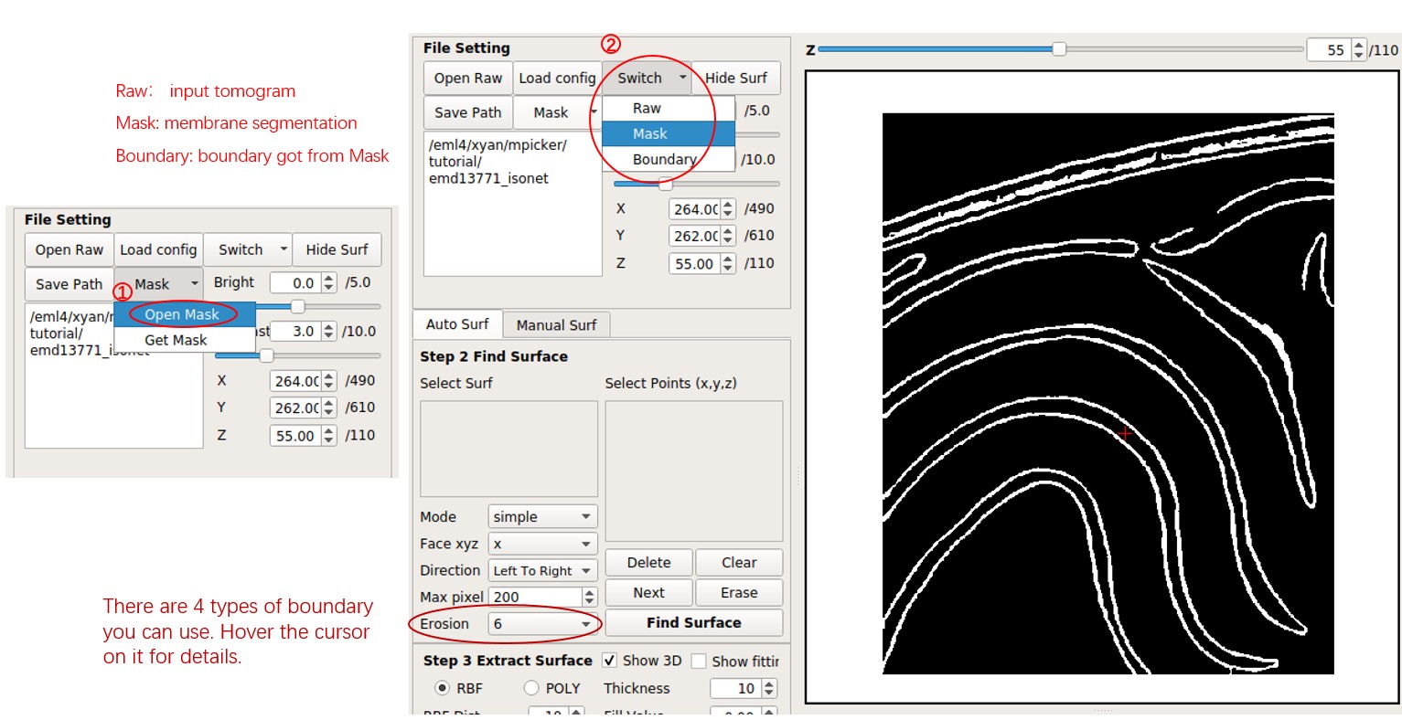
Press Mask, select Open Mask, and choose the segmentation file seg_post_id0_thres_0.60_gauss_0.50_voxel_150.mrc.

MPicker will load it and calculate its boundary, which may take some time. It will generate a new file tutorial/emd13771_isonet/my_boundary_6.mrc.

Toggle between the raw tomogram, segmentation, or boundary by pressing Switch and choosing Raw, Mask, or Boundary. The boundary is the essential component for subsequent tasks, serving as the point cloud representation of the entire surface.

Separate a Surface

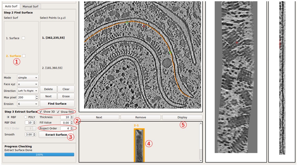
Move the red cross to a point near the membrane surface by left-clicking it. Then press Shift + S or right-click and choose Save as Reference. The point will be added to the Select Points list, marked by green arrows. Press Find Surface to separate the surface near the point.

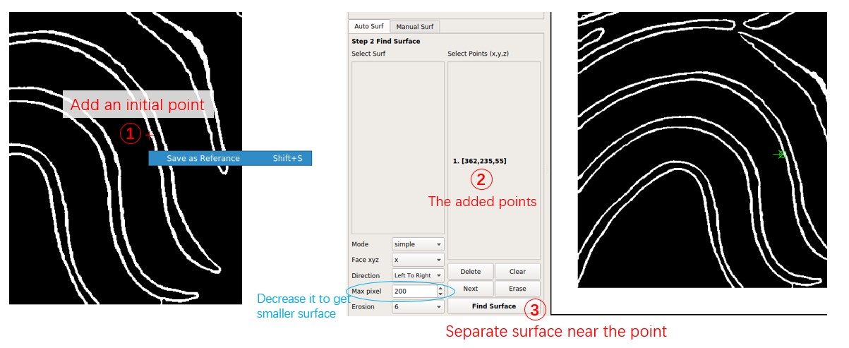
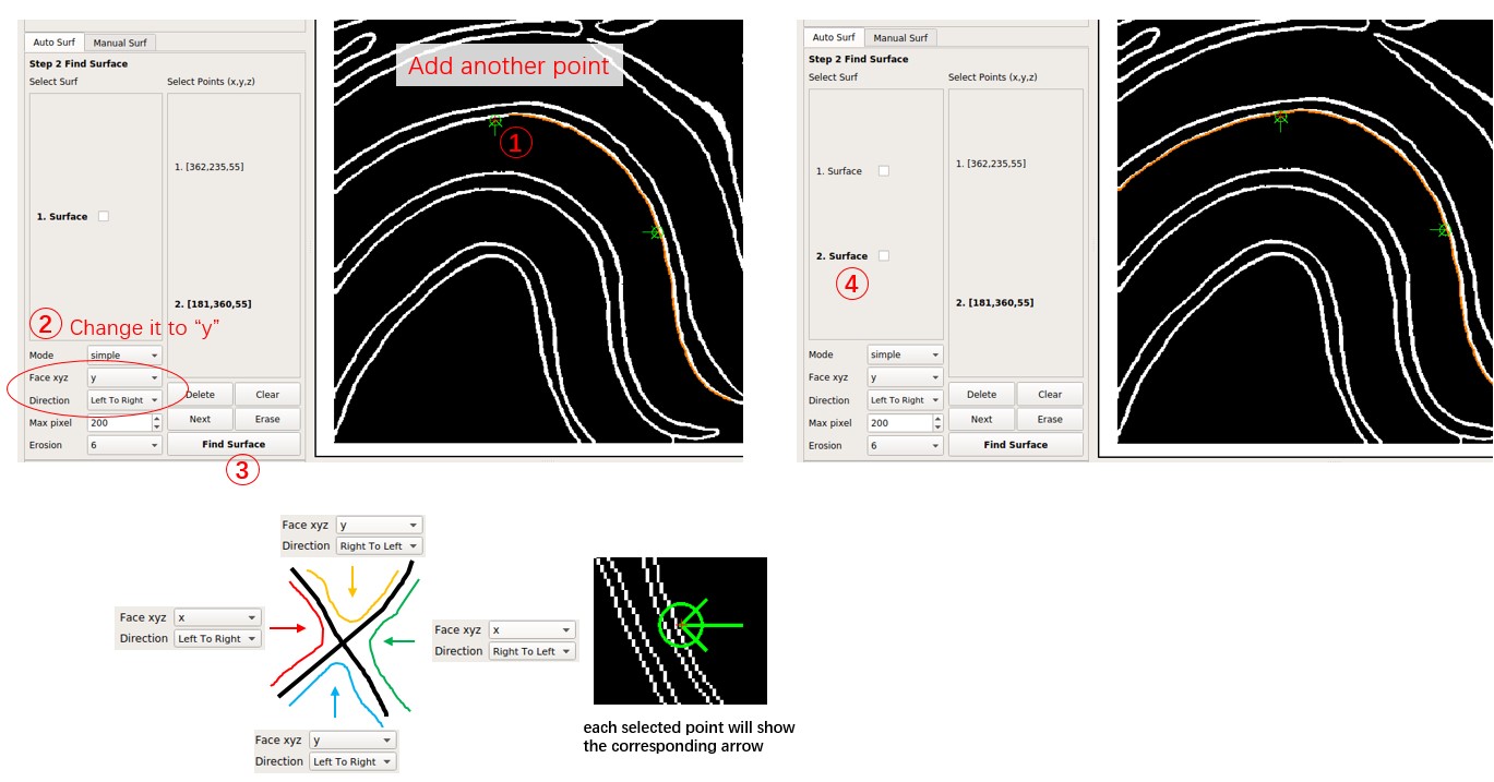
Now the first separated surface is shown in orange. The orange line ends at the top because the Face xyz of the point is x, indicating that it separates the surface perpendicular to the x-axis, or the surface can be represented as x = f(y,z).

To add the top region to the surface, add another point based on the first surface. Click near the membrane surface on the top region, press Shift + S as before, and change Face xyz to y. Each point can have different Face xyz and Direction, determining where the line extends when facing forks. Press Find Surface to separate the second surface.

Note that the Select Points list of the surface in the Select Surf list will be fixed. Add new points based on the selected surface and press Find Surface to get a new surface. Remember to press Clear before adding points for a completely new surface. To delete the selected point, press Delete.

Switch between different surfaces by clicking them in the Select Surf list, and delete them by right-clicking and choosing Delete Selected.

For a boundary with low quality, indicating many forks and discontinuities, it is advisable to decrease Max pixel and choose more points at different places on the membrane surface.

Flatten a Surface

Select the second surface by clicking 2. Surface. Change Project Order to 4, indicating MPicker will project it onto a fourth-order polynomial cylinder. Increase thick for a thicker flattened tomogram.

Press Extract Surface to flatten the membrane; this process takes about 5 seconds. A flattened tomogram labeled 2-1 will be obtained. Select it by clicking, then press Display to view the flattened tomogram on the right side.

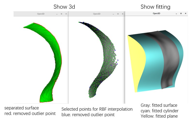
Check Show 3D and Show fitting to observe the intermediate process in 3D. Note that viewing it remotely, for example, through an SSH connection, may limit visibility due to OpenGL reasons, but it won't affect the result.

Modify parameters and press Extract Surface again to obtain another flattened tomogram of this surface, for example, 2-2. Experiment by changing Project Order to 1 to observe the result of projecting it onto a plane rather than a cylinder. In general, increasing Project Order may solve issues if the result appears strange.

Check the Result

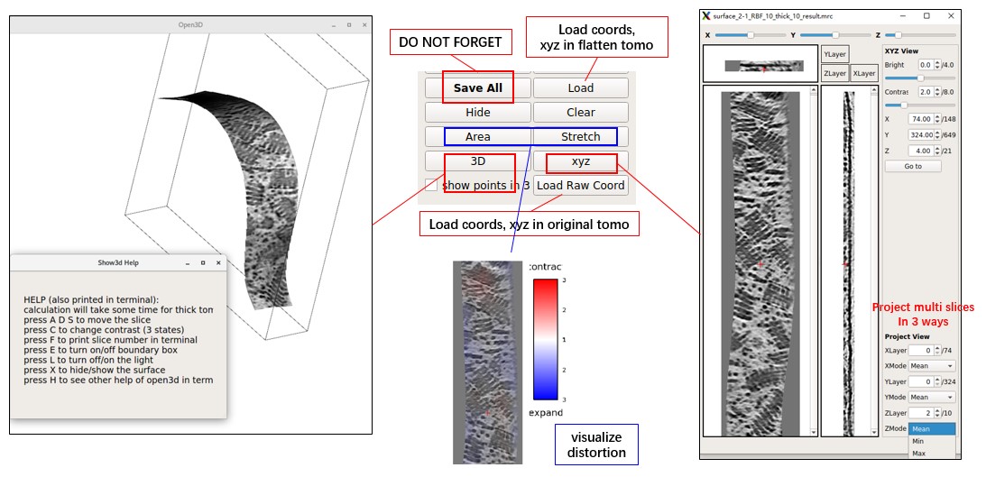
Examine the flattened tomogram on the right side. Adjust the image contrast using the Bright and Contrast spinbox. Move the red cross by left-clicking on the image, adjusting the spinbox of xyz coordinates, or pressing arrow keys. Note that the red cross on the left side (raw tomogram) will move correspondingly. These two crosses indicate the same location.

The main GUI will display XY and YZ slices. View both XY, YZ, and XZ slices and project multiple slices in a new window by pressing xyz. To assess the distortion caused by flattening, press Area or Stretch. To view XY slices in 3D space (without distortion), press 3D.

Output Files of MPicker

MPicker should generate some files and folders as shown below. The most important ones are emd13771_isonet.config, emd13771_isonet/*/*_result.mrc, and emd13771_isonet/*/*_InterpCoords.txt. Others can be ignored for now for non-advanced users.

--tutorial
  -- emd13771_isonet.config
  -- emd13771_isonet
    -- my_boundary6.mrc
    -- surface_1_emd13771_isonet 
      ...
    -- surface_2_emd13771_isonet
      -- surface_2.config
      -- surface_2_surf.mrc.npz
      -- surface_2-1.config
      -- surface_2-1_RBF_10_thick_10_convert_coord.npy
      -- surface_2-1_RBF_10_thick_10_result.mrc
      -- surface_2-1_RBF_10_thick_10_SelectPoints.txt
      -- surface_2-1_RBF_InterpCoords.txt
      ...
    -- manual_1_emd13771_isonet
      -- manual_1.config
      -- manual_1_surf.txt
      -- manual_1-1.config
      -- manual_1-1_RBF_10_thick_10_convert_coord.npy
      -- manual_1-1_RBF_10_thick_10_result.mrc
      -- manual_1-1_RBF_10_thick_10_SelectPoints.txt
      -- manual_1-1_RBF_InterpCoords.txt
    -- memseg
        -- seg_raw_id0.mrc
        -- seg_post_id0_thres_0.60_gauss_0.50_voxel_150.mrc
        ...

• emd13771_isonet is the folder that contains all results of MPicker.

• emd13771_isonet.config is used to reload the result. Continue working in MPicker next time with:

  Mpicker_gui.py --config path_to/emd13771_isonet.config &
  

  The config file can also be loaded by pressing Load Config after opening the GUI. The config file saves the absolute path of the input tomogram, membrane segmentation, and boundary file. If the result folder and config file are relocated, ensure that they remain in the same directory. Also, remember to update the file paths in the config file, including the path for my_boundary6.mrc.

• my_boundaryxxx.mrc is the boundary file calculated from segmentation. MPicker calculates it because a membrane is thick. By using only one of the two boundary surfaces of a membrane, MPicker can flatten the membrane with higher accuracy.

• Each separated surface will have its folder, such as surface_2_emd13771_isonet, which is the folder of 2.Surface. The file surface_2.config records parameters MPicker used to separate it from the boundary. surface_2_surf.mrc.npz is the separated surface, and conversion between .npz file and .mrc file can be done by the script Mpicker_convert_mrc.py. MPicker converts .mrc to .npz to save space.

• Each separated surface can be flattened into more than one flattened tomogram, such as 2-1, 2-2. They are all saved in one folder. The .config file records the parameters used to flatten. The _result.mrc file is the flattened tomogram itself. The _convert_coord.npy file records the relationship of coordinates between the flattened tomogram and the original tomogram. If x, y, z in the flattened tomogram correspond to Rx, Ry, Rz in the original tomogram, and they start from 0, then Rx, Ry, Rz can be obtained by Rz, Ry, Rx = numpy.load("xxx.npy")[:, z, y, x]. The _InterpCoords.txt file records the points MPicker finally used for RBF interpolation, and more points can be used by decreasing RBF Dist and vice versa. The _SelectPoints.txt file records all information of particles picked in the flattened tomogram. See Particle Picking by Hand for details.

• If surfaces are separated by manually labeled points, see Flatten Membrane Without Segmentation for details, then each surface will also have its folder, such as manual_1_emd13771_isonet. It doesn't have a .mrc.npz file because it is not from segmentation, but it has a file to record manually labeled points such as manual_1_surf.txt. Other files are the same as those in the surface separated from segmentation.

• If membrane segmentation is done in MPicker, see Generate Membrane Segmentation for details, then a folder memseg will be created, which saves all results of segmentation. Note that seg_raw_id0.mrc cannot be used as the Mask because it is not a binary segmentation (with only 0 or 1 as its value).

Particle Picking by Hand

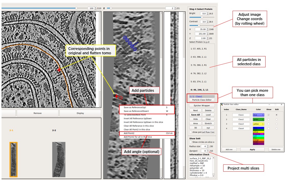
Now particles can be manually picked in the flattened tomogram. Position the red cross by left-clicking and press S to save the position (or right-click and select Save as Reference). Note that there is a distinction between Up (S) and Down (W), but it can be ignored (just press S) if particle orientation is not a concern. Refer to the image below for a more intuitive understanding.

Remember to press Save All before quitting or displaying another flattened tomogram.

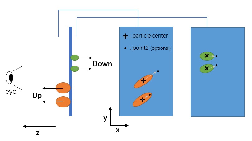
MPicker will record the corresponding membrane normal vector for each picked particle, but the normal vector can have two options, Up or Down, depending on which side of the membrane the particle is on.

A position can also be added as "point2" for a selected particle, enabling complete determination of the particle's orientation (grey arrow as the x-axis and the norm vector as the z-axis). To add point2 for a particle, move to the same xy slice as the selected particle, position the red cross, and press Ctrl+A (or right-click and press Add Point2).

To select a picked particle, double-click on a particle in the xy slice, and its circle will turn red. Ensure that the center of the circle is on this xy slice (cross is displayed). A particle can also be selected by clicking on the ones listed on the right side.

Particles can also be picked in the flattened tomogram (a file ending with _result.mrc) using other software if preferred. To load the result into MPicker, simply load the coordinate file (a txt file with 3 columns as x y z, starting from 1) by pressing Load. If particles are already picked in the original tomogram, load the coordinates by pressing Load Raw Coord and check them in the flattened tomogram. Particles outside of the flattened tomogram will be ignored. Coordinate conversion between the original and flattened tomogram can also be performed using the script Mpicker_convert_coord.py.

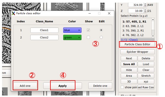
More than one class of particle can be picked together. Press Particle Class Editor, and then press Add one to add a new class. Select which class to edit (pick particles) and which classes to display. Then press Apply to use it. The color and name for each class can be changed, but MPicker will only save the index into _SelectPoints.txt. Note that pressing Delete one will not delete the data of particles; it only controls the display. For example, if some particles are picked in Class2 and then the Class2 is deleted, the gui will display 1/2: Class1, 2 means the particle in the saved data with the highest index is 2. They can be seen again if class2 is added back.

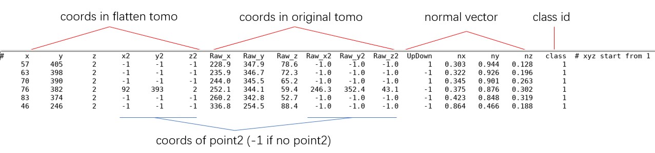
The information of picked particles for each flattened tomogram is saved in files ending with _SelectPoints.txt. For surface 2-1, it is tutorial/emd13771_isonet/surface_2_emd13771_isonet/surface_2-1_RBF_10_thick_10_SelectPoints.txt. Below is what it looks like.

All _SelectPoints.txt of one tomogram can be merged and converted into Euler angles using the script Mpicker_particles.py. For example:

Mpicker_particles.py --input emd13771_isonet --out_mer merge.txt --out_ang angle.txt

It will merge all _SelectPoints.txt files in the result folder emd13771_isonet into merge.txt and then convert it to angle.txt. Below is what angle.txt looks like. X Y Z are the coordinates of particles in the original tomogram, and the definition of rot tilt psi is the same as rlnAngleRot rlnAngleTilt rlnAnglePsi in Relion.

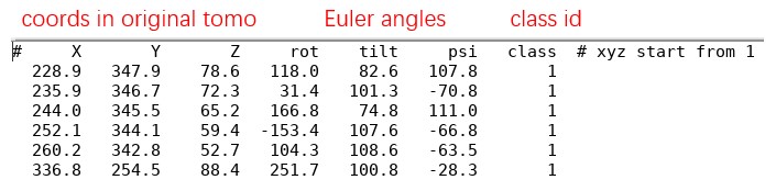
Note: Normal vectors can only decide tilt and psi, so the rot of particles without point2 will be filled with a random angle. The rot of all particles without point2 can also be set to 0 by adding --fill_rot 0. Type Mpicker_particles.py -h for details. Note that UpDown can be 1 (Up) or -1 (Down), so the real normal vectors should be UpDown * (nx, ny, nz).

Generate Membrane Segmentation

This step can be skipped if a segmentation is already available. To run membrane segmentation, ensure the computer has at least one GPU, and the full version of MPicker is installed (see installation instructions for details).

First, press Mask and choose Get Mask, and MPicker will open a new window.

Next, press Run in the left half of the window. (Change GPU id to 0,1 and adjust batch size and threads to 4 if there are 2 GPUs.)

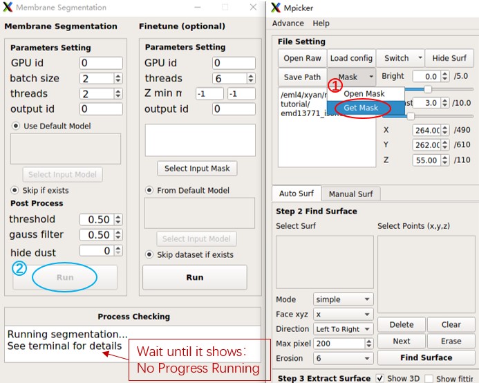
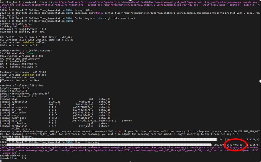
Wait until it finishes. This process takes about 4 minutes (one GeForce RTX 2080 Ti was used here). The terminal will display something like this:

The results will be stored in xxx/tutorial/emd13771_isonet/memseg:

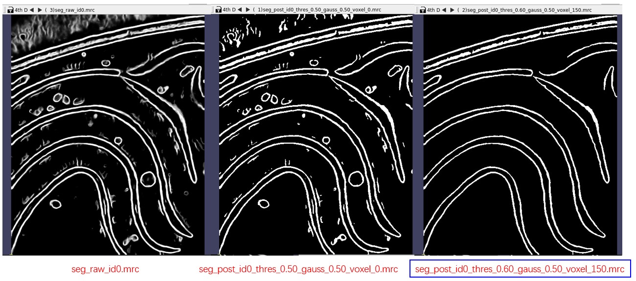
• seg_raw_id0.mrc: raw segmentation from neural network, continuous map, ranging from 0 to 1
• seg_post_id0_thres_0.50_gauss_0.50_voxel_0.mrc: result of post-process, binary mask, 0 or 1, takes much less time than raw seg

Verify the results using 3dmod or other preferred software. The result of post-process (binary mask) is what is needed. Adjust parameters of post-process if necessary. Here, threshold was increased to 0.6 to remove weak signals and hide dust was changed to 150 to eliminate small connected components.

Then press Run on the left side again. A new result will be obtained soon, as it only performs post-processing this time. It will generate a new file seg_post_id0_thres_0.60_gauss_0.50_voxel_150.mrc, which should be similar to the segmentation contained in the tutorial folder.

Now, close the segmentation window and return to the main window.

Flatten Membrane Without Segmentation

In case a suitable segmentation is not available, Load Membrane Segmentation and Separate a Surface can be skipped by labeling membranes by hand.

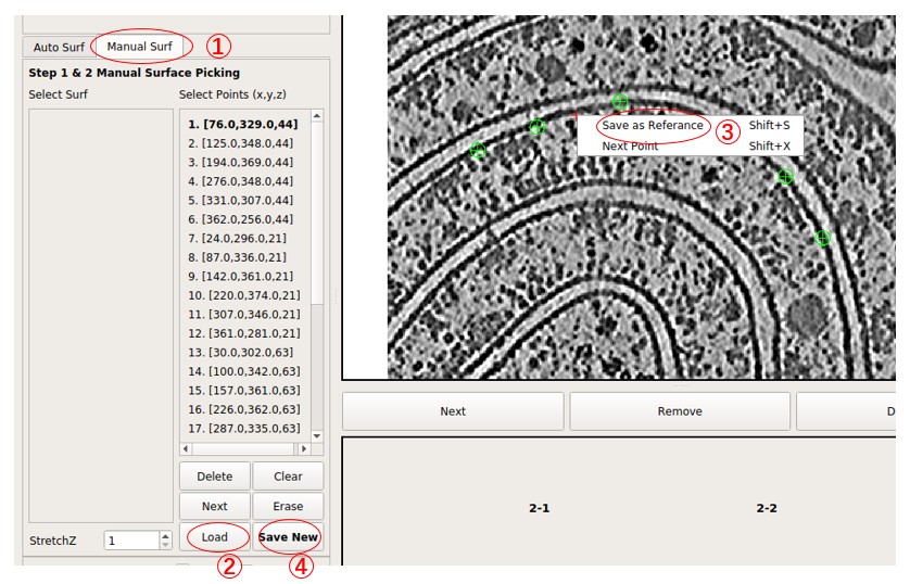
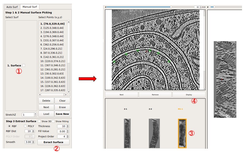
Select the tab Manual Surf instead of Auto surf, then press Load to load the coordinate file manual_surf.txt, which contains 29 manually labeled membrane positions. Labels can also be added manually. Similar to what was done in Separate a Surface, move the red cross to a point on the membrane by left-clicking it, then press Shift + S or right-click and choose Save as Reference to save it. Then, it will be added to the Select Points list. The added points are indicated by green circles. Press Save New to save these points as a new surface.

Next, press Extract Surface to flatten the membrane, and a flattened tomogram called M1-1 will be obtained. Select it by clicking it. Then, press Display to view the flattened tomogram on the right side. The membrane is not as flattened as in surface 2-1 because the number of points is much less than what was used in surface 2-1. However, it is sufficient to visualize large membrane proteins. More points can be added to improve the result.

In general, RBF Dist can be decreased to 1 in this mode to preserve all points added. It decides the minimal distance (in pixels) between points used at last. Also, Project Order should not be high if the number of points is small.

To see which points were used for surface 2-1 (separated from segmentation), press Clear to clear current points, and then press Load to load file emd13771_isonet/surface_2_emd13771_isonet/surface_2-1_RBF_InterpCoords.txt, which should contain about 305 points.