MPicker Manual

Welcome to MPicker! Here are detailed instructions about GUI. Prior to reviewing this manual, it is recommended to go through the tutorial.

Load Tomogram

• Click the Open Raw button to choose a tomogram for processing.
• Click the Save Path button to select a save folder. (A config file and a folder will be created for each tomogram under the save folder.)

• Alternatively, you can use the following commands:

  • --raw ... to select a raw file.
  • --out ... to set a save path.

  

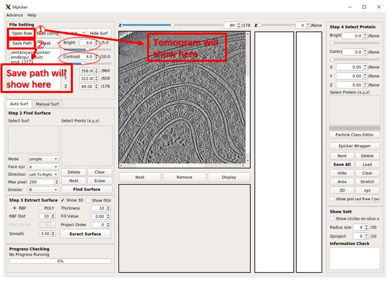
  Adjust the brightness and contrast as needed. Generally, Bright=0 and Contrast<=5 work well. You can easily adjust any value in the spinbox (brightness, contrast, x, y, z, etc.) by rolling the wheel on it.

Get Mask (Membrane Segmentation)

• Click the Mask button on the upper-left of the main GUI.
• Choose Open Mask to load an existing membrane segmentation mask.
• Alternatively, choose Get Mask to generate segmentation using a pre-trained AI in a new GUI.

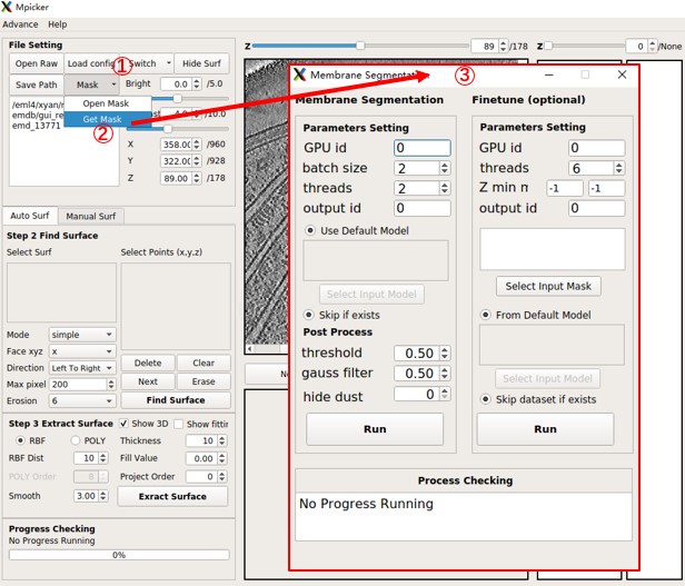
Membrane Segmentation GUI:

The Membrane Segmentation GUI has Parameters Setting and Post Process sections (ignore the right half).

• Parameter Setting generates segmentation with continuous values (raw seg) by AI. These parameters mainly affect computation time.
• Post Process generates a binary segmentation (values of 0 or 1) to determine the final mask (important). Results are saved in the "memseg" folder under the output folder for the tomogram.

Parameters Setting:

• GPU id: Specifies which GPUs to use (e.g., 0 for a single GPU, 0,1 for two GPUs).
• batch size: A good starting point is 2 * number_of_gpus (means each GPU processes 2 batches at once).
• threads: Can be equal to batch size, or less than it.
• output id: If the raw seg file with this id already exists, this part will be skipped. The ID can be any alphanumeric string.

Post Process:

• threshold: Voxels in raw seg larger than this value will be set to 1; smaller values will be set to 0.
• gauss filter: Applies a Gaussian filter to raw seg with this sigma before use threshold.
• hide dust: Removes small connected components in each 2D slice and then in 3D. The value is the pixel number cutoff in 2D, and 100 times this value is the voxel number cutoff in 3D. 100 is a good try, and use 0 to skip it.

Press the Run button on the left side to start the segmentation. After completion, choose Open Mask in the main GUI to load the result (e.g., seg_post_id0_thres_0.50_gauss_0.50_voxel_0.mrc).

Step 2: Find Surface

There are two methods for surface detection: Auto Surf (requires a mask) and Manual Surf (doesn't require a mask but need to mark multiple points manually).

Auto Surf

Auto Surf automatically separates a surface from the mask boundary. User need to select one or several points on ONE surface. Follow these steps:

1. Click on Mask and Open Mask to load the mask for the raw tomogram. MPicker generates the boundary when you input a mask.
2. Click on Switch to toggle between the raw tomogram, mask, and boundary. This is for display purposes, and you can select points in any mode, but only points near the boundary are valid.
3. Scroll and drag the mouse on the view to inspect the tomogram. Use the left mouse button to locate the coordinates.
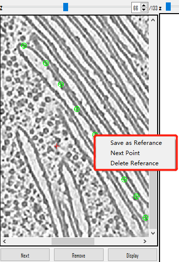
4. Right-click and choose Save as reference, or use the shortcut key Shift+S. The coordinates will appear on the left.
5. If the selected points are unsatisfactory, delete them using the Delete button, or right-click near the selected point and choose Delete Reference, or use the shortcut key Shift+D to delete the last selected point.
6. Adjust the parameters for better results. You can use the default settings for the first time and make adjustments based on the outcomes.
7. Press Find Surface to locate one surface from the selected points. You can add or delete points on the base of the selected surface without changing its recorded points to generate a new surface. Remember to press Clear before selecting a new surface.

Right-click menu in view:

• Save as Reference (Shortcut Key=Shift+S): Save the selected points for surface finding.
• Next Point (Shortcut Key=Shift+X): Select the next point (Same as Next Button above).
• Delete Reference (Shortcut Key=Shift+D): Delete the points that are selected (Same as Delete above).

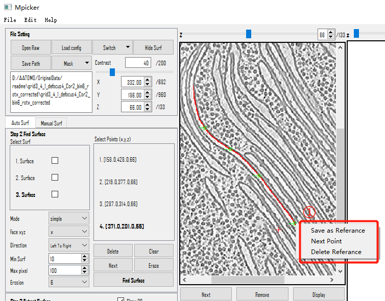
Parameters:

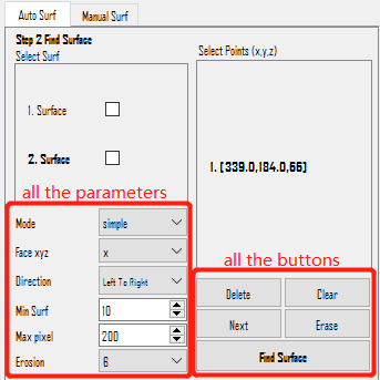
• Mode: Generally, use "simple". Other mode may get more area with less points but is unstable.
• Face xyz: The orientation the surface faces. It can be x, y, or z, although membranes perpendicular to z are rare in general tomogram.
• Direction: How the surface will be extended on the folk point.
• Max pixel: The largest length to extend from given points.
• Erosion: The method to generate a boundary from the mask.

Consider a boundary with X shape (it will happen when seg is not good enough), different combination of Face xyz and Direction will separate different part of the X. Each point can have different xyz and direction.

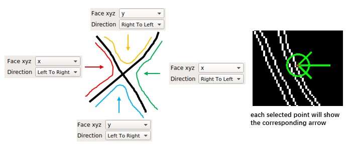
Buttons below Select Points scrollArea:

• Delete: Delete the points that are selected (bold in Select Points scrollArea above).
• Clear: Delete all the points.
• Next: Select the next point.
• Erase: Currently has no function.
• Find Surface: Run the Surface Finding.

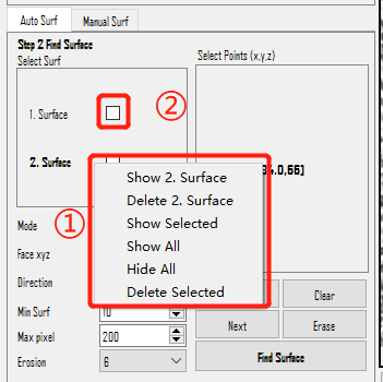
Right-click menu in Select Surf scrollArea:

• Show xx. Surface: Displays this result surface in the view. This action does NOT mean selecting the surface. To select a surface, left-click on it and making it bold.
• Delete xx. Surface: Permanently deletes this result surface.
• Show Selected: Displays all the selected result surfaces. It will show all the surfaces whose checkboxes (②) are checked.
• Show All: Displays all the result surfaces. It will also check all the checkboxes.
• Hide All: Closes all the result surfaces that are currently displayed. This action will also clear all the checks in the checkboxes.
• Delete Selected: Deletes all the selected result surfaces. It will delete all the surfaces whose checkboxes are checked.

Manual Surf

Manual Surf means manually labeling surfaces by selecting several points on ONE surface. The section doesn't have specific parameters but requires a substantial number of manually selected points (e.g., selecting 5 points in one slice and doing this for 5 slices results in a total of 25 points).

1. Switch to Manual Surf mode by clicking on Manual Surf.
2. Right-click and choose save as reference to add points. Alternatively, use Shortcut Key Shift+S, and the coordinate will appear on the left.
3. If the selected points are unsatisfactory, delete them using the Delete button, or right-click near the selected point and choose Delete Reference, or use Shortcut Key Shift+D to delete the last selected point.
4. Press Save New to store the selected points as a new surface. You can add or delete points based on the selected surface without changing its recorded points to generate a new surface. Remember to press Clear before starting to select a new surface.
5. You can also load a txt file by pressing Load if you already have coordinates from elsewhere.

Right-click menu in view:

• Save as Reference (Shortcut Key=Shift+S): Save the selected points to indicate the surface.
• Next Point (Shortcut Key=Shift+X): Select the next point (Same as Next Button above).
• Delete Reference (Shortcut Key=Shift+D): Delete the points that are selected (Same as Delete above).

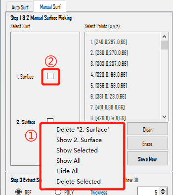
Right-click menu in Select Surf scrollArea is the same as that in Auto Surf.

Step 3: Extract Surface

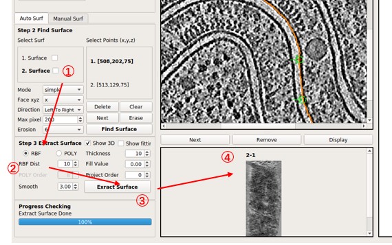
There are two methods that can be used for Surface Extraction: Polynomial surface fitting (short for POLY) and Radial Basis Function surface interpolation (short for RBF).

1. Select one surface from step 2.
2. Choose either the RBF or POLY Mode, then adjust other parameters (Show 3D and Show fitting will not influence the result).
3. Press Extract Surface to obtain the result in the scrollArea.

Parameters Introduction

Extract Surface: Flatten ONE surface based on RBF or POLY.

Here are all the parameters:

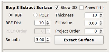
• RBF: The radio button is checked to choose RBF Mode (thin-plate spline interpolation). Generally, it flattens the membrane better, but the surface may not be as smooth.
• POLY: The radio button is checked to choose POLY Mode. The result is smooth enough (polynomial function), but it might be hard to flatten membranes perfectly.
• RBF Dist: Only used in RBF mode. It is the distance between sampling points on the surface, in pixels. A smaller distance will use more points and be slower. Typically, 10 is small enough. For Manual Surf, you can set it to 1 to use nearly all points.
• Smooth: Only used in RBF mode. Determines the error allowed in the interpolation. Too small Smooth or too small RBF Dist may cause remarkable distortions in slices far from the center layer (caused by unsmoothness of the surface). A value of 3 is generally used.
• POLY Order: Only used in POLY mode. It is the order of the polynomial when doing the surface fitting. A higher order may flatten the surface better but can produce an awful boundary. Typically, less than 10 is used.
• Thickness: Number of slices above and under the center layer. So the final thickness (in pixels) of the flattened tomogram will be 2 * Thickness + 1.
• Fill Value: Fills the value to the pixel in the flattened tomogram where there is no corresponding pixel in the original tomogram. 0 is a special value here, which means fill by the mean value (not 0).
• Project Order: Order of the polynomial when doing the cylinder fitting. The surface will be projected onto a cylinder to reduce the distortion of flattening. 4 is a good try for an opened cylinder. -1 means a closed ellipse cylinder. Set to 0 or 1 if you think your surface is not a cylinder at all.
• Show3D: Whether or not to show some intermediate results. It will display the input surface (from step 2) in 3D, the result of outlier points removing, and which points are selected for RBF interpolation. It is helpful if you want to adjust parameters. It needs Open3D and may fail for remote connections (such as ssh -X).
• Show fitting: Whether or not to show the result of surface fitting, as well as the cylinder and plane.

Scroll Area

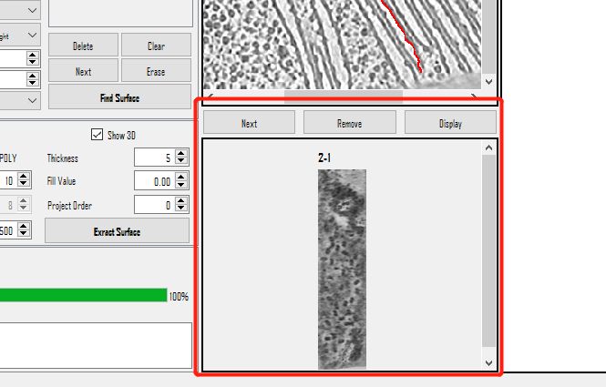
Users can process and choose the result tomogram from scroll area.

• Next: Move on to the next result tomogram.
• Remove: Permanently delete the result tomogram.
• Display: Check the result tomogram on the right side.

Step 4: Select Proteins

Check the Result

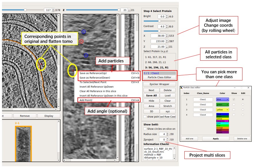
• Left-click to locate the coordinates.
• Right-click to add, delete, or check the next selected points.
• Double-click to select a point.
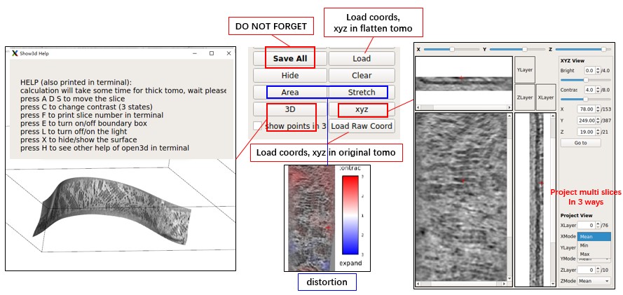
• Don't forget to press Save all to save the picked particles to a txt file. (MPicker saves and loads coordinates using xyz starting from 1.)

Parameter Introduction & Keyboard Shortcuts

Here are the parameter introduction and keyboard shortcuts:

• Select Protein(x,y,z): The scrollArea stores all the selected protein coordinates. L(left) R(right) means up or down, 1 2 means whether it contains angle information (you need 2 points to get an angle).
• Next: Check the next selected proteins.
• Delete: Delete the selected proteins.
• Save All: Save all proteins into the file. Press it before switching to another flattened tomogram; it will NOT save automatically.
• Load: Load coordinates of proteins from a file with 3 columns (x, y, z of one particle per row, starting from 1). If more than 3 columns, it will ignore the rest.
• Load Raw Coord: Similar to Load, but uses coordinates in the original tomogram. It converts input coordinates to the coordinates in the flattened tomogram, ignoring the part outside the flattened tomogram.
• Hide: Hide all the selected proteins on the view (helps users check tomogram density).
• Clear: Clear all coordinates in the current class. Will not save to the file unless you press Save all.
• 3D: Check out the 3D mode of the current result tomogram.
• xyz: Check out the xyz mode of the current result tomogram.
• Radius size: Change the circle of the selected protein to help users have a better understanding of selected proteins. The circle will be shown in multiple slices like a sphere (not a real sphere), unless you check Show circles on-slice only.
• Area and Stretch: Show area deformation and angle deformation in color.
• Epicker Wrapper is a wrapper of Epicker. You need to install Epicker first to use it. It is a deep learning software for particle picking, but there is no pre-trained model. You need to generate some trainset and train a model first. You can try labeling 100 particles for training initially.

Here are the main keyboard shortcuts:

• Save as Reference Up (Key=S): Pick the particle if the Z-coordinate of the protein extracellular domain is larger than the membrane (protein in the upper half part).
• Save as Reference Down (Key=W): Pick the particle if the Z-coordinate of the protein extracellular domain is smaller than the membrane (protein in the lower half part).
  • We distinguish Up or Down just in case you want to use the normal vector of the membrane for the calculation of subtomo average. You can ignore the difference between Up and Down if you just need coordinates.
• Next Point (Key=X): Check the next selected proteins (Same as Next). The red cross will move to the current particle if not already positioned there.
• Delete Reference (Key=CTRL+D): Delete the selected points (Same as Delete).
• Add Point2 (Key=CTRL+A): Add orientation information for the selected particle by adding another point. The second point will connect to the selected particle and form a line to label the orientation.
• Delete Point2 (Key=CTRL+Z): Delete Point2 for the selected particle, and the line will disappear.

Output Files

• Each surface in Step 2 has a dedicated folder, and each surface can generate more than one flattened tomogram.
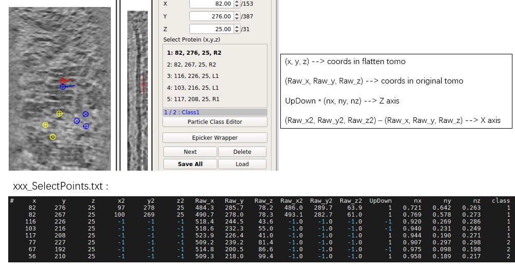
• Each flattened tomogram has a text file ending with _SelectPoints.txt, which saves the results of particle picking.
• The MRC file of the flattened tomogram ends with _result.mrc.
• The NPY file ending with _convert_coord.npy saves the conversion from flattened coordinates to original coordinates. It is a 4D array, z_raw, y_raw, x_raw = array[:, z-1, y-1, x-1] + 1.

For example, taking the tomogram named grid3_4_1_corrected.mrc:

--<results_dir>
  -- grid3_4_1_corrected                                  (Stores all the results and processing history)
      -- my_boundary6.mrc                                 (Edge detection of the raw tomogram) 
      -- manual_1_grid3_4_1_corrected 
         -- manual_1.config                               (Config file for manual surface finding)
         -- manual_1_surf.txt                             (Selected points)
         -- manual_1-1.config                             (Config file for manual surface extraction)
         -- manual_1-1_RBF_10_thick_5_result.mrc          (Result tomogram)
         -- manual_1-1_RBF_10_thick_5_convert_coord.npy   (Coordinate conversion numpy)
         -- manual_1-1_RBF_10_thick_5_SelectPoints.txt    (Selected protein coordinates)
         -- ...
      -- manual_2_grid3_4_1_corrected
      -- ...
      -- surface_1_grid3_4_1_corrected
         -- surface_1.config                              (Config file for auto surface finding)
         -- surface_1_surf.mrc.npz                        (Surface finding result tomogram)
         -- surface_1-1.config                            (Config file for auto surface extraction)
         -- surface_1-1_RBF_10_thick_5_result.mrc         (Result tomogram)
         -- surface_1-1_RBF_10_thick_5_convert_coord.npy  (Coordinate conversion numpy)
         -- surface_1-1_RBF_10_thick_5_SelectPoints.txt   (Selected protein coordinates)
      -- surface_2_grid3_4_1_corrected
      -- ...
  -- memseg                                               (Stores all the mask results)
      -- seg_raw_id0.mrc                                  (Raw segmentation result, **DO NOT USE IT AS MASK**)
      -- seg_post_id0_thres_0.50_gauss_0.50_voxel_100.mrc (Processed mask, This is the INPUT MASK)
      -- ...
  -- grid3_4_1_corrected.config                           (You can reload all the history by loading the config file in GUI)

Additional File

• All python files starting with Mpicker_ are executable scripts. Here are some of them, and you can find more details about the scripts by using the --help option:
  • Mpicker_particles.py: Merges all _SelectPoints.txt files of all flattened tomograms in a raw tomogram. It can also convert them to Euler angles.
  • Mpicker_2dprojection.py: Projects particles along the normal vector from the raw tomogram to get 2D images. It can also generate corresponding 2dCTF from a given 3dCTF. (for Class2D)
  • Mpicker_3dctf.py: Generate a coarse 3dCTF with missing wedge.
  • Mpicker_convert_coord.py: Converts coordinates between raw tomograms and flattened tomograms.
  • Mpicker_add_coord.py: Add xyz coordinates to an existed _SelectPoints.txt file.
  • Mpicker_mrcnpy2mrc.py: Generates a flattened tomogram from a given flattened tomogram and a new raw tomogram. (For example, if you already have a flattened tomogram from a tomogram treated with isonet, you can directly get a flattened tomogram from an untreated tomogram.)
  • Mpicker_convert_mrc.py: Converts .mrc.npz files to .mrc so that you can edit it and replace the old one. (The surface is stored as .npz to save space)
• imagev2.ui, help.ui, check.ui, memseg.ui... are for GUI design. Users can edit them using PyQt-Designer.